|
| (1) |
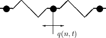
where q(n,t) is the displacement of the n-th particle from its equilibrium position, p(n,t) is its momentum (mass m = 1), and V (r) is the interaction potential.
Restricting the attention to finitely many particles (e.g., by imposing periodic
boundary conditions) and to the harmonic interaction V (r) =  , the equations of
motion form a linear system of differential equations with constant coefficients. The
solution is then given by a superposition of the associated normal modes. Around 1950 it
was generally believed that a generic nonlinear perturbation would yield to
thermalization. That is, for any initial condition the energy should eventually be equally
distributed over all normal modes. In 1955 Enrico Fermi, John Pasta, and Stanislaw
Ulam carried out a seemingly innocent computer experiment at Los Alamos, [5], to
investigate the rate of approach to the equipartition of energy. However, much to
everybody’s surprise, the experiment indicated, instead of the expected thermalization, a
quasi-periodic motion of the system! Many attempts were made to explain this result but
it was not until ten years later that Martin Kruskal and Norman Zabusky, [18], revealed
the connections with solitons (see [1] for further historical information and a pedagogical
discussion).
, the equations of
motion form a linear system of differential equations with constant coefficients. The
solution is then given by a superposition of the associated normal modes. Around 1950 it
was generally believed that a generic nonlinear perturbation would yield to
thermalization. That is, for any initial condition the energy should eventually be equally
distributed over all normal modes. In 1955 Enrico Fermi, John Pasta, and Stanislaw
Ulam carried out a seemingly innocent computer experiment at Los Alamos, [5], to
investigate the rate of approach to the equipartition of energy. However, much to
everybody’s surprise, the experiment indicated, instead of the expected thermalization, a
quasi-periodic motion of the system! Many attempts were made to explain this result but
it was not until ten years later that Martin Kruskal and Norman Zabusky, [18], revealed
the connections with solitons (see [1] for further historical information and a pedagogical
discussion).
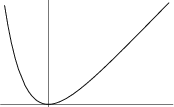
This had a big impact on soliton mathematics and led to an explosive growth in the last decades. In particular, it led to the search for a potential V (r) for which the above system has soliton solutions. By considering addition formulas for elliptic functions, Morikazu Toda came up with the choice V (r) = e-r + r - 1. The corresponding system is now known as the Toda equation, [17].
The equation of motion in this case reads explicitly
 p(n,t) p(n,t) | = - = e-(q(n,t)-q(n-1,t)) - e-(q(n+1,t)-q(n,t)), = e-(q(n,t)-q(n-1,t)) - e-(q(n+1,t)-q(n,t)), | ||
 q(n,t) q(n,t) | =  = p(n,t). = p(n,t). | (2) |
The important property of the Toda equation is the existence of so called soliton solutions, that is, pulslike waves which spread in time without changing their size or shape and interact with each other in a particle-like way. This is a surprising phenomenon, since for a generic linear equation one would expect spreading of waves (dispersion) and for a generic nonlinear force one would expect that solutions only exist for a finite time (breaking of waves). Obviously our particular force is such that both phenomena cancel each other giving rise to a stable wave existing for all time!
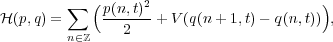
In fact, in the simplest case of one soliton, you can easily verify that this solution is given by
 | (3) |
with κ,γ > 0 and σ  {±1}.
{±1}.
|
It describes a single bump traveling through the crystal with speed σ sinh(κ)∕κ and width proportional to 1∕κ. In other words, the smaller the soliton the faster it propagates. It results in a total displacement 2κ of the crystal.
However, this is just the tip of the iceberg and can be generalized to the N-soliton solution
 | (4) |
where
 | (5) |
with κj,γj > 0 and σj {±1}. The case N = 1 coincides with the one soliton solution
from above and asymptotically, as t →∞, the N-soliton solution can be written as a sum
of one-soliton solutions. However, the solitones undergo nonlinear interactions. For
example, if a faster soliton overtakes a slower one, after the interaction took
place, the faster one is shifted backward and the slower one is shifted forwared a
bit.
Two examples with N = 2 are depicted below.
|
|
Historically such solitary waves were first observed by the naval architect John Scott Russel [14], who followed the bow wave of a barge which moved along a channel maintaining its speed and size (see the review article [13] for further information).
The importance of these solitary waves is that they constitute the stable part of the solutions arising from arbitrary short range initial conditions and can be used to explain the quasi-periodic behaviour found by Fermi, Pasta, and Ulam. In fact, the classical result discovered by Zabusky and Kruskal [18] states that every ”short range” initial condition eventually splits into a number of stable solitons and a decaying background radiation component.
|
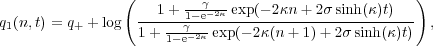
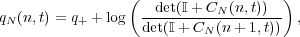
This is illustrated in Figure 6 which shows the numerically computed solution q(n,t)
corresponding to the initial condition q(n,0) = δ0,n, p(n,0) = 0 at some large time
t = 130. You can see the soliton region | | > 1 with two single soliton on the very left
respectively right and the oscillatory region |
| > 1 with two single soliton on the very left
respectively right and the oscillatory region | | < 1 where there is a continuous
displacement plus some small oscillations which decay like t-1∕2 and are asymptotically
given by
| < 1 where there is a continuous
displacement plus some small oscillations which decay like t-1∕2 and are asymptotically
given by
 | (6) |
where z0 = eiθ0 is a slow variable depending only on  and the functions T0(z0), ν(z0),
Φ0(z0), and δ(z0) are explicitly given in terms of the scattering data associated with the
initial data.
and the functions T0(z0), ν(z0),
Φ0(z0), and δ(z0) are explicitly given in terms of the scattering data associated with the
initial data.
Existence of soliton solutions is usually connected to complete integrability of the system, and this is also true for the Toda equation. To see that the Toda equation is indeed integrable we introduce Flaschka’s variables [6]
 | (7) |
and obtain the form most convenient for us
 a(t) a(t) | = a(t) b+(t) - b(t) b+(t) - b(t) , , | ||
 b(t) b(t) | = 2 a(t)2 - a-(t)2 a(t)2 - a-(t)2 . . | (8) |
 | (9) |
Note that if q(n,t) → q± sufficiently fast as n →±∞, the converse map is given by
 | (10) |
Moreover, q(n,t) → q±, p(n,t) → 0 as |n|→∞ corresponds to a(n,t) → ,
b(n,t) → 0.
,
b(n,t) → 0.
To show complete integrability it suffices to find a so-called Lax pair [11], that is, two operators H(t), P(t) in ℓ2(ℤ) such that the Lax equation
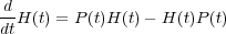 | (11) |
is equivalent to (8). One can easily convince oneself that the right choice is
| H(t) | = a(t)S+ + a-(t)S- + b(t), | ||
| P(t) | = a(t)S+ - a-(t)S-, | (12) |
 are unitarily equivalent (cf. [15,
Thm. 12.4]):
are unitarily equivalent (cf. [15,
Thm. 12.4]):
Theorem 1. Let P(t) be a family of bounded skew-adjoint operators, such that t P(t)
is differentiable. Then there exists a family of unitary propagators U(t,s) for P(t), that
is,
P(t)
is differentiable. Then there exists a family of unitary propagators U(t,s) for P(t), that
is,
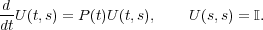 | (13) |
Moreover, the Lax equation (11) implies
 | (14) |
This result has several important consequences. First of all it implies global existence of solutions of the Toda lattice. In fact, considering the Banach space of all bounded real-valued coefficients (a(n),b(n)) (with the sup norm), local existence follows from standard results for differential equations in Banach spaces. Moreover, Theorem 1 implies that the norm ∥H(t)∥ is constant, which in turn provides a uniform bound on the coefficients of H(t),
 | (15) |
Hence solutions of the Toda lattice cannot blow up and are global in time (see [15, Sect. 12.2] for details).
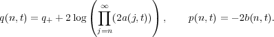
Second, it provides an infinite sequence of conservation laws expected from a completely integrable system. Indeed, if the Lax equation (11) holds for H(t), it automatically also holds for H(t)j. Taking traces shows that
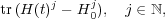 | (16) |
is an infinite sequence of conserved quantities, where H0 is the operator corresponding to
the constant solution a0(n,t) =  , b0(n,t) = 0 (it is needed to make the trace converge).
Introducing a suitable symplectic structure, they can be shown to be in involution as well
([8, Sect. 1.7]). For example,
, b0(n,t) = 0 (it is needed to make the trace converge).
Introducing a suitable symplectic structure, they can be shown to be in involution as well
([8, Sect. 1.7]). For example,
tr H(t) - H0 H(t) - H0 | = ∑
n ℤb(n,t) = - ℤb(n,t) = - ∑
nℤp(n,t) and ∑
nℤp(n,t) and | ||
tr H(t)2 - H
02 H(t)2 - H
02 | = ∑
nℤb(n,t)2 + 2(a(n,t)2 - ) = ) =   (p,q) (p,q) | (17) |
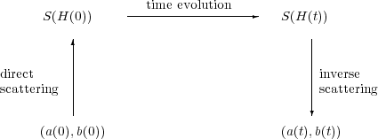
These observations pave the way for a solution of the Toda equation via the inverse
scattering transform originally invented by Gardner, Green, Kruskal, and Miura [7] for
the Korteweg–De Vries equation (see [15, Sect. 13.4] for the case of the Toda lattice). In
particular, Theorem 1 implies that the operators H(t), t , are unitarily equivalent
and that the spectrum σ(H(t)) is independent of t. Now the general idea is to find
suitable spectral data S(H(t)) for H(t) which uniquely determine H(t). Then equation
(11) can be used to derive linear evolution equations for S(H(t)) which are easy to
solve. In our case these data will be the so called scattering data and the formal
procedure (which can be thought of as a nonlinear Fourier transform) is summarized
below:
The inverse scattering step will be done by reformulating the problem as a
Riemann–Hilbert factorization problem. This Riemann–Hilbert problem will
then be analyzed using the method of nonlinear steepest descent by Deift and
Zhou [2] (which is the nonlinear analog of the steepest descent for Fourier type
integrals).
For further information on the history of the steepest descent method, which was inspired by earlier work of Manakov [12] and Its [9], and the problem of finding the long-time asymptotics for integrable nonlinear wave equations, we refer to the survey by Deift, Its, and Zhou [3].
More information on the Toda lattice can be found in the monographs by Faddeev and Takhtajan [4], Gesztesy, Holden, Michor, and Teschl [8], Teschl [15], or Toda [17]. Here we followed the review article by Teschl [16] and Krüger and Teschl [10]. A much more comprehensive guide to the literature can be found in Section 1.8 of [8].
[1] T. Dauxois, M. Peyrard, and S. Ruffo, The Fermi–Pasta–Ulam ’numerical experiment’: history and pedagogical perspectives, Eur. J. Phys. 26, S3–S11 (2005).
[2] P. Deift and X. Zhou, A steepest descent method for oscillatory Riemann–Hilbert problems, Ann. of Math. (2) 137, 295–368 (1993).
[3] P. A. Deift, A. R. Its, A. R., and X. Zhou, Long-time asymptotics for integrable nonlinear wave equations, in “Important developments in soliton theory”, 181–204, Springer Ser. Nonlinear Dynam., Springer, Berlin, 1993.
[4] L. Faddeev and L. Takhtajan, Hamiltonian Methods in the Theory of Solitons, Springer, Berlin, 1987.
[5] E. Fermi, J. Pasta, S. Ulam, Studies of Nonlinear Problems, Collected Works of Enrico Fermi, University of Chicago Press, Vol.II,978–988,1965. Theory, Methods, and Applications, 2nd ed., Marcel Dekker, New York, 2000.
[6] H. Flaschka, The Toda lattice. I. Existence of integrals, Phys. Rev. B 9, 1924–1925 (1974).
[7] C. S. Gardner, J. M. Green, M. D. Kruskal, and R. M. Miura, A method for solving the Korteweg-de Vries equation, Phys. Rev. Letters 19, 1095–1097 (1967).
[8] F. Gesztesy, H. Holden, J. Michor, and G. Teschl, Soliton Equations and Their Algebro-Geometric Solutions. Volume II: (1+1)-Dimensional Discrete Models, Cambridge Studies in Advanced Mathematics 114, Cambridge University Press, Cambridge, 2008.
[9] A.R. Its, Asymptotics of solutions of the nonlinear Schrödinger equation and isomonodromic deformations of systems of linear differential equations, Soviet Math. Dokl. 24, 452–456 (1981).
[10] H. Krüger and G. Teschl, Long-time asymptotics of the Toda lattice for decaying initial data revisited, Rev. Math. Phys. 21:1, 61–109 (2009).
[11] P. D. Lax Integrals of nonlinear equations of evolution and solitary waves, Comm. Pure and Appl. Math. 21, 467–490 (1968).
[12] S. V. Manakov, Nonlinear Frauenhofer diffraction, Sov. Phys. JETP 38:4, 693–696 (1974).
[13] R. S. Palais, The symmetries of solitons, Bull. Amer. Math. Soc., 34, 339–403 (1997).
[14] J. S. Russel, Report on waves, 14th Mtg. of the British Assoc. for the Advance of Science, John Murray, London, pp. 311–390 + 57 plates, (1844).
[15] G. Teschl, Jacobi Operators and Completely Integrable Nonlinear Lattices, Math. Surv. and Mon. 72, Amer. Math. Soc., Rhode Island, 2000.
[16] G. Teschl, Almost everything you always wanted to know about the Toda equation, Jahresber. Deutsch. Math.-Verein. 103, no. 4, 149–162 (2001).
[17] M. Toda, Theory of Nonlinear Lattices, 2nd enl. ed., Springer, Berlin, 1989.
[18] N. J. Zabusky and M. D. Kruskal, Interaction of solitons in a collisionless plasma and the recurrence of initial states, Phys. Rev. Lett. 15, 240–243 (1965).