

The Optimization Test Environment is an interface to solve optimization problems efficiently using different solver routines. It is designed as a tool for both developers of solver software and practitioners who just look for the best solver for their specific problem class.
The software is developed by Dr. Ferenc Domes, Dr. Martin Fuchs, Prof. Hermann Schichl, and Prof. Arnold Neumaier. It enables users to: Choose and compare diverse solver routines; organize and solve large test problem sets; select interactively subsets of test problem sets; perform a statistical analysis of the results, automatically produced as LaTeX, PDF, and JPG output. The Optimization Test Environment is free to use for research purposes.
DOWNLOAD The Optimization Test Environment
Testing is a crucial part of software development in general, and hence also in optimization. Unfortunately, it is often a time consuming and little exciting activity. This naturally motivated us to increase the efficiency in testing solvers for optimization problems and to automatize as much of the procedure as possible.
Optimization Solver Benchmarks
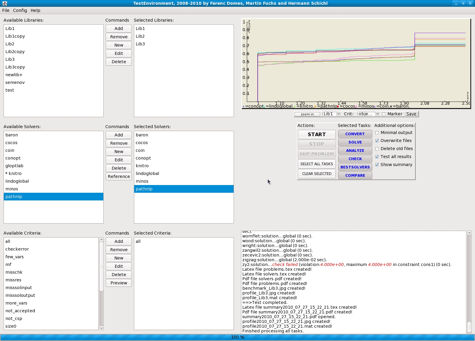
The procedure typically consists of three basic tasks: organize possibly large test problem sets (also called test libraries); choose solvers and solve selected test problems with selected solvers; analyze, check and compare the results. The Optimization Test Environment is a graphical user interface (GUI) that enables to manage the first two tasks interactively, and the third task automatically.
Thus the Optimization Test Environment is particularly designed for users who seek to:The first point concerns a situation in which the user wants to improve parameters of a particular solver manually, see, e.g., GloptLab. The second point is interesting in many real-life applications in which a good solution algorithm for a particular problem is sought. The third point targets general benchmarks of solver software. It often requires a selection of subsets of large test problem sets (based on common characteristics, like similar problem size), and afterwards running all available solvers on these subsets with problem class specific default parameters, e.g., timeout. Finally all tested solvers are compared with respect to some performance measure.
In the literature, such comparisons typically exist for black box problems only, see, e.g., the large online collection H. Mittelmann. Benchmarks, 2009, mainly for local optimization. Since in most real-life applications models are given as black box functions, it is popular to focus comparisons on this problem class. However, the popularity of modeling languages like AMPL and GAMS, that formulate objectives and constraints algebraically, is increasing. Thus first steps are made towards comparisons of global solvers using modeling languages, e.g., on the gamsworld website Gamsworld. Performance tools, which offers test sets and tools for comparing solvers with interface to GAMS.
One main difficulty of solver comparison is to determine a reasonable criterion to measure the performance of a solver. Our concept of comparison is to count for each solver the number of global numerical solutions found, and the number of wrong and correct claims for the solutions. Here we consider the term global numerical solution as the best solution found among all solvers. We also produce several more results and enable the creation of performance profiles.
Further rather technical difficulties come with duplicate test problems, the identification of which is an open task for future versions of the Optimization Test Environment.
A severe showstopper of many current test environments is that it is uncomfortable to use them, i.e., the library and solver management are not very user-friendly, and features like automated LaTeX table creation are missing. Test environments like CUTEr provide a test library, some kind of modeling language (in this case SIF) with associated interfaces to the solvers to be tested. The unpleasant rest is up to the user. However, our interpretation of the term test environment also requests to analyze and summarize the results automatically in a way that it can be used easily as a basis for numerical experiments in scientific publications. A similar approach is used in Libopt, available for Unix/Linux, but not restricted to optimization problems. It provides test library management, library subset selection, solve tasks, all as more or less user-friendly console commands only. Also it is able to produce performance profiles from the results automatically. The main drawback is the limited amount of supported solvers, restricted to black box optimization.
Our approach to developing the Optimization Test Environment is inspired by the experience made during the comparisons, in which the Coconut Environment benchmark is run on several different solvers. The goal is to create an easy-to-use library and solver management tool, with an intuitive GUI, and an easy, multi-platform installation. Hence the core part of the Optimization Test Environment is interactive. We have dedicated particular effort to the interactive library subset selection, determined by criteria such as a minimum number of constraints, or a maximum number of integer variables or similar. Also the solver selection is done interactively.
The modular part of the Optimization Test Environment is mainly designed as scripts without having fixed a script language, so it is possible to use Perl, Python, etc. according to the preference of the user. The scripts are interfaces from the Optimization Test Environment to solvers. They have a simple structure as their task is simply to call a solve command for selected solvers, or simplify the solver output to a unified format for the Optimization Test Environment. A collection of already existing scripts for several solvers, including setup instructions, is available at the Download the Optimization Test Environment page of this website. We explicitly encourage people who have implemented a solve or analyze script for the Optimization Test Environment to send it to the authors who will add it to the website. By the use of scripts the modular part becomes very flexible. For many users default scripts a convenient, but just a few modifications in a script allow for non default adjustment of solver parameters without the need to manipulate code of the Optimization Test Environment. This may significantly improve the performance of a solver.
As the problem representation we use Directed Acyclic Graphs (DAGs) from the Coconut Environment. We have decided to choose this format as the Coconut Environment already contains automatic conversion tools from many modeling languages to DAGs and vice versa. The Optimization Test Environment is thus independent from any choice of a modeling language. Nevertheless benchmark problem collections, e.g., given in AMPL such as COPS, can be easily converted to DAGs. The analyzer of the COPS test set allows for solution checks and iterative refinement of solver tolerances. The DAG format enables us to go in the same direction as we are also automatically performing a check of the solutions. With the DAG format, the present version of the Optimization Test Environment excludes test problems that are created in a black box fashion.
Finally, the Optimization Test Environment is managing automated tasks which have to be performed manually in many former test environments. These tasks include an automatic check of solutions, and the generation of LaTeX tables that can be copied and pasted easily in numerical result sections of scientific publications. As mentioned we test especially whether global solutions are obtained and correctly claimed. The results of the Optimization Test Environment also allow for the automated creation of performance profiles.