1.1.2 Halftone Approximation

If we cannot display all the required intensity levels (e.g. on a printer) we need a trick using the spatial integration that our eyes performs: In normal light the eye can only detect about one arc minute ($1/60$ degree). This is called VISUAL ACUITY. Thus instead of gray dots a small black disk with radius varying according to the blackness $1-I$ is printed. Usually, for newspaper 60-80 and for magazines 150-200 different radiuses are used. This process is called HALFTONING.

Figure: Halftoning

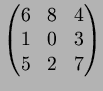
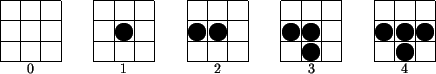
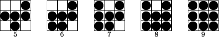
For computers this is implemented as CLUSTERED-DOT ORDERED DITHERING, e.g. the following patterns are used for each pixel of intensity $0\dots 9$:

Figure:

Figure: Clustered-dot ordered dithering

Figure: Clustered-dot ordered dithering

This can be described by a dither matrix

$$\begin{pmatrix} 6 & 8 & 4 \\ 1 & 0 & 3 \\ 5 & 2 & 7 \\ \end{pmatrix}$$

saying that in order to display intensity $I$ one should turn on all those pixels whose value in this matrix is less than $I$. It is chosen in such a way, that visual artifacts are avoided:

• Growth sequence to minimize contour effects, i.e. the pattern are subsets of each other (hence the name ordered). They start in the center and expand towards the boundary.
• Keep the one's adjacent to each other (hence the name clustered dot), but this is not necessary for monitors.

For high-quality reproduction we need an $8\times 8$ (64 gray levels) or even a $10\times 10$ matrix and thus quite a hight resolution.

If such a high resolution is not available one can use ERROR DIFFUSION: There we use fewer intensity levels than desired, but we distribute the errors $I - I_i$ to the neighboring pixels with the following weights:

$$\xymatrix{ &\bullet\ar@{->}[0,1] \ar@{->}[1,1] \ar@{->}[1,0] \ar@{->}[1,-1] &7/16 \\ 3/16 &5/16 &1/16 \\ }$$

Figure: 8 colors with Floyd-Steinberg error diffusion

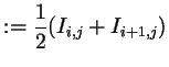
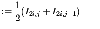
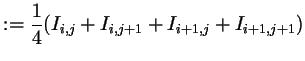
A similar trick can be used for enlarging a picture by taking interpolation values to neighboring pixels as intermediate values. E.g. for doubling the size of the picture one inserts new rows and columns and takes as new values

$$I_{2i,2j}' :=I_{i,j} I_{2i+1,2j}' :=\frac12(I_{i,j}+I_{i+1,j})$$

$$I_{2i,2j+1}' :=\frac12(I_{2i,j}+I_{2i,j+1})\qquad I_{2i+1,2j+1}' :=\frac14(I_{i,j}+I_{i,j+1}+I_{i+1,j}+I_{i+1,j+1})$$

This way one avoids that small square-size pixels can be seen. Disadvantage is that some blurring occurs.

Figure: Enlarged versus enlarged with diffusion